Passing data to cf-plot
Using cf-python - cf compliant data
Data is generally passed to cf-plot via cf-python as a 2-dimensional field.
import cf
import cfplot as cfp
f=cf.read('cfplot_data/ggap.nc')
f is now an list of 4 fields.
[<CF Field: air_temperature(time(1), pressure(23), latitude(160), longitude(320)) K>,
 <CF Field: eastward_wind(time(1), pressure(23), latitude(160), longitude(320)) m s**-1>,
 <CF Field: geopotential(time(1), pressure(23), latitude(160), longitude(320)) m**2 s**-2>,
 <CF Field: northward_wind(time(1), pressure(23), latitude(160), longitude(320)) m s**-1>]
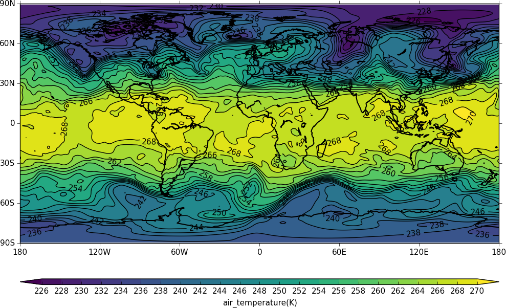
To contour data a 2 dimensional field is needed. In the case below we select the 500mb temperature with the cf subspace method.
f[0].subspace(pressure=500)
<CF Field: air_temperature(time(1), pressure(1), latitude(160), longitude(320)) K>
cfp.con(f[2].subspace(pressure=500))
To mean the field use the cf collapse function:
f[0].collapse( 'mean','longitude')
<CF Field: air_temperature(time(1), pressure(23), latitude(160), longitude(1)) K>
cfp.con(f[2].collapse( 'mean','longitude'))

Using cf-plot with non-cf compliant data
Although newer model and reanalyis products are generally cf compliant there is a considerable amount of data being used that is of varying degrees of cf compliance.
Example 1
In this locally processed ERA40 reanalysis field there is a distinct lack of standard names. Even the long names are somewhat terse - p for pressure for example.
f=cf.read('cfplot_data/ggap.nc')[2]
f
<CF Field: geopotential(time(1), pressure(23), latitude(160), longitude(320)) m**2 s**-2>
We can still slice and plot the data by inspecting the dimensions of the field:
f.items()
{'dim2': <CF DimensionCoordinate: latitude(160) degrees_north>,
 'dim3': <CF DimensionCoordinate: longitude(320) degrees_east>,
 'dim0': <CF DimensionCoordinate: time(1) days since 1964-01-21 00:00:00>,
 'dim1': <CF DimensionCoordinate: pressure(23) mbar>}
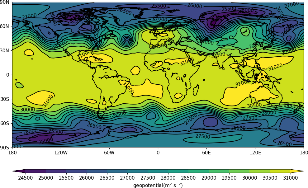
We see that dim1 is the pressure coordinate and can select the 700mb level and contour that.
f.item('dim1').array
array([ 1000.,   925.,   850.,   775.,   700.,   600.,   500.,   400.,
        300.,   250.,   200.,   150.,   100.,    70.,    50.,    30.,
        20.,    10.,     7.,     5.,     3.,     2.,     1.], dtype=float32)


f.subspace(dim1=700)
<CF Field: geopotential(time(1), pressure(1), latitude(160), longitude(320)) m**2 s**-2>


cfp.con(f.subspace(dim1=700))
Example 2
In this dataset there are neither standard or long names.
f=cf.read('cfplot_data/gdata.nc')[0]
<CF Field: ncvar:temp(ncvar:p(22), ncvar:lat(73), ncvar:lon(145)) >
We can still slice and plot the data as below.
f.items()
{'dim2': <CF DimensionCoordinate: ncvar:lon(145)>,
'dim0': <CF DimensionCoordinate: ncvar:p(22)>,
'dim1': <CF DimensionCoordinate: ncvar:lat(73)>}

f.item('dim0').array
array([  1.00000000e+03,   7.00000000e+02,   5.00000000e+02,
      3.20000000e+02,   2.15000000e+02,   1.50000000e+02,
      1.00000000e+02,   7.00000000e+01,   5.00000000e+01,
      3.20000000e+01,   2.00000000e+01,   1.50000000e+01,
      1.00000000e+01,   7.00000000e+00,   5.00000000e+00,
      3.20000005e+00,   2.00000000e+00,   1.50000000e+00,
      1.00000000e+00,   6.99999988e-01,   5.00000000e-01,
      3.00000012e-01], dtype=float32)
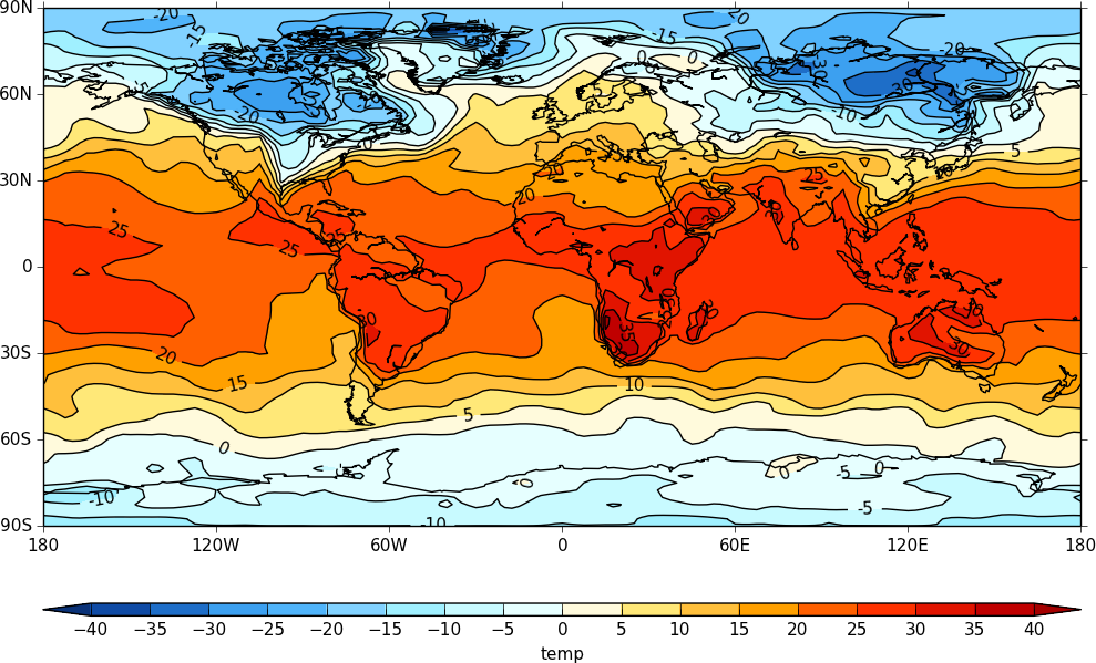
So to plot the 1000mb temperature we would use:
cfp.con(f.subspace(dim0=1000))
Passing data via arrays
cf-plot can also make contour and vector plots by passing data arrays.
import cfplot as cfp
from netCDF4 import Dataset as ncfile
nc = ncfile('cfplot_data/tas_A1.nc')[0]
lons=nc.variables['lon'][:]
lats=nc.variables['lat'][:]
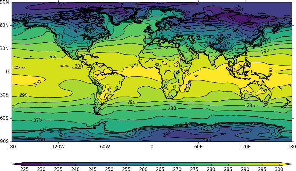
temp=nc.variables['tas'][0,:,:]
cfp.con(f=temp, x=lons, y=lats)
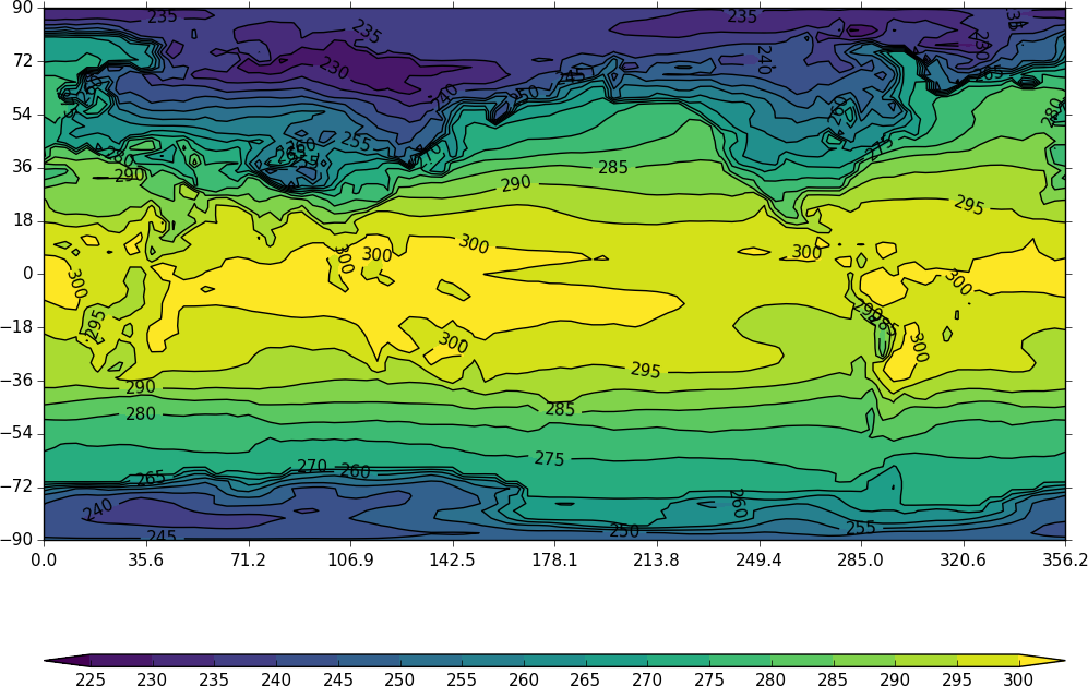
The contouring routine doesn't know that the data passed is a map plot. This can be explicitly set with the ptype flag to con.
cfp.con(f=temp, x=lons, y=lats, ptype=1)
Other types of plot are: